Latest Entries »

This was quite a lengthy project: A fully running Commodore Amiga500 emulator. It has all the necessary features to run most of the games from back in the days.
It is basically a simulation of the Amiga’s main-processor, co-processor, blitter, displaychips, soundchips, ROM, RAM, Disk drives, DMA and all those things.
It comes with a debugging panel and a simple disassembler as can be seen from the screen-shot. And yes: “Chuck Rock” runs like a charm, including the great music and everything… 😉

I think it’s about time for a round of “Pinball Dreams”…

This rendering was produced by evaluating the famous mandelbrot fractal, but instead of just counting the number of iterations for each pixel I wanted to draw the positions of the full sequence/trajectory (until bailout) of points from each starting point. Since the iterative function is quite chaotic the points within the sequence scatter all over the image in a very unpredictable fashion.
The challenge of rendering this image lies in the fact that when displaying a tiny region of the overall space only a tiny amount of points will fall in the view and billions of them will fall somewhere else where they don’t contribute to the final rendering at all. In order to not waste billions of iterations to get just a few rendered pixels I used the Metropolis/Hastings algorithm. This technique will “mutate” past trajectories (or paths) which did successfully fall in the view in order to produce (to a high chance) more points which will also fall in that view. This algorithm works well, because similar starting points will produce similar trajectories (but trajectories will diverge in some exponential fashion). This technique is also quite useful when computing global illumination of 3D scenes as this is sampling-wise quite a similar problem.

This was an attempt to simulate the structure-forming process in the universe.
3 million particles were initially placed at random positions within a sphere of space so they appear as a shapeless, homogenous fog.
Now every particle interacts with all others by gravity. Just by that they would implode into a single dense region. To avoid this a “vacuum-force” is applied which pushes each particle outwards in proportion to its location from the center. This counter-acts the collapse caused by the gravitational field and instead the particles converge into this sponge-like pattern. Where filaments connect into dense regions would be the location of star-clusters (and within those you would see galaxies), but for each “star-cluster” there are only a few particles left (around 40), so you cannot see more detail than that with “just” 3 million particles.
The pattern actually matches quite well to serious super-computer calculations done by astrophysicist.
I did the simulation in 3D as well, but basically the same pattern emerges – just 3D (but its not so nicely visualizable and many more particles would be needed).


I was always fascinated by the visual beauty and mind-blowing force of large-scale explosions. And since nobody should get hurt, the computer was once again the weapon of choice.
In the upper image you can see the simulation view showing flow dynamics and the lower image shows a sequence of final renderings.
The simulation is done using grid-based Navier-Stokes fluid dynamics and additional Kolmogorov-turbulence to compute the dynamics of airflow.
Now plenty of particles can advect along this flow and are rendered each frame with a custom volume renderer.

I created this image by raytracing using a distance function approximation of the Mandelbulb fractal. The rendering of the fractal is 3 dimensional and it has a lot of depth which is not really visible, because the degree of detail is infinte at all levels and therefore it is impossible to extract depth-cues from the details.
For that reason I’ve extended the rendering to produce stereoscopic outputs which greatly enhances the appearence of the actual shape. It is quite stunning to browse through different regions in full stereo-3D.

You can download a hi-res anaglyph stereo-rendering here (note: left/right is swapped due to my oddly swapped glasses)

This video shows realtime raytracing of procedural volumetric data (warped metaballs) including reflection, shading, 2 lights, shadows and ambient-occlusion.
Computation is done in CUDA and executed on a GeForce285GTX. The video quality is not so great as something went wrong with the frame rate. I didn’t have any good grabber at hand.

This is a test of displaying VirtualReality on a regular LCD-monitor.
The simple 3D scene appears as a hologram on the screen. You can easily look around obstacles just as if the screen would be a window or portal instead of a flat surface showing an image.
It has been filmed with an iPod so the quality isn’t all that great and the colors distorted a little which yields stronger ghosting, but I think you can still clearly see the effect.

NOTE: My Red/Cyan 3D-glasses seem to be a little odd as they have the RED glass on the RIGHT eye. Usually this seems to be the other way around, so if your 3D glasses have the red glass on the left just wear them up-side-down for a proper 3d effect.

This is part of my “artificial perception” project.

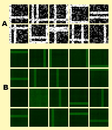
An image (16×16 pixels) is generated which consists of 8 horizontal and 8 vertical white bars with each being either shown or hidden by chance. This means there is a total of 2^16=65536 patterns possible. Additionally the generated image is degraded by adding 50% noise to make recognition harder (this ultimately increases the number of possible patterns to infinite).

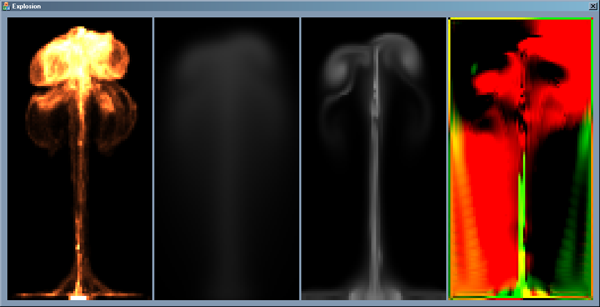
(A) shows a small subset of these input patterns.

Now these patterns are presented one-by-one (no batch processing) to a system consisting of 20 artificial neurons (amount is arbitrarily choosable) and each neuron updates its synapses by my new learning-rule.
The idea is that the system “learns to understand” the pattern-generating process and instead of trying to remember all possible patterns (65536 without noise and close to infinity for the noisy ones) which is completely unfeasable due to size constraints it extracts each bar seperately (even tho they are almost never shown in isolation, but always in combination with other bars). It does so as every pattern experienced so far can be reconstructed from these (2*8) separate bars.

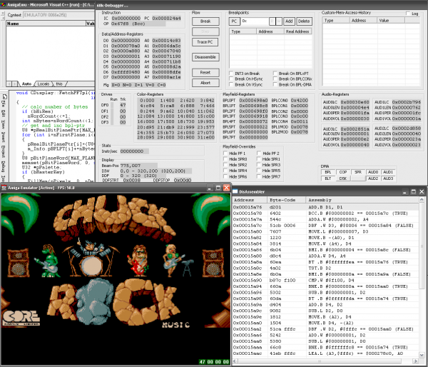
(B) shows that 4 of the 20 neurons will remain unspecialized while the other 16 will specialize towards one of the 2*8 bars.

Also as you can see each neuron’s specialization in (B) is mainly free of noise (and therefore the whole percept) even tho a great amount of noise was inherent in each presented pattern.

This results in a 16-bit code which is the optimal solution to represent all patterns in a compact manner.

Computational complexity is O(N²) where N is the number of neurons. Memory complexity is just O(N).
Complexity is NOT dependent on the amount of patterns shown (or possible).
This should be one of the fastest online learning methods for this test without storing or processing previously experienced patterns.

After being in the wanting-but-not-spending-time-on-it phase for several years, I finally present: My own website. Yeehaa…

Here I’ll show some outcomes of my past and recent projects I’ve worked on in my spare-time. This includes natural science related research and computer simulations, computer graphics, sound & music and other.

I’ll add descriptions and other projects in the next days.

To find out who I am take a look at the About-page.


I hope you like it.